How an Instrument Gets Made Here
The shop method, end to end: an instrument is drawn as engineering sheets, assembled by hand, measured at microsecond scale, cataloged bend by bend, and only then played. The thing being engineered is controlled ruin.
This shop breaks video on purpose, and everything about that sentence is technical. A glitch that arrives whenever it feels like it, at whatever depth it feels like, is weather — you can film it, but you can’t play it. The work here is turning a failure mode into an instrument: the wreckage has to arrive on cue, at a set depth, and come back the same tomorrow. Precision is not the opposite of the aesthetic. Precision is what makes the aesthetic repeatable.
Every instrument passes through the same five stages.
1. Draw
An instrument exists on paper before it exists in copper, and stays on paper while it’s being built. The working format is a 13×19 engineering sheet — monospace, one page, printed and marked up in pen. A sheet carries the power tree, the bus map, the connector table, numbered footnotes for every decision that had a fork in it, and an open-items column that stays honest about what isn’t solved yet.
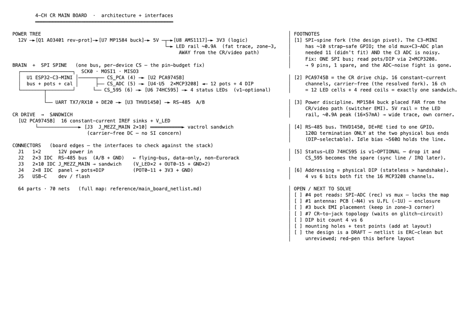 FIG. 1 — Architecture sheet for a four-channel control board: power tree, a single SPI spine, the drive stage, connectors at the board edges. The open-items column ends by calling the design a draft to be red-penned before layout. The sheet is where mistakes get caught while they are still ink.
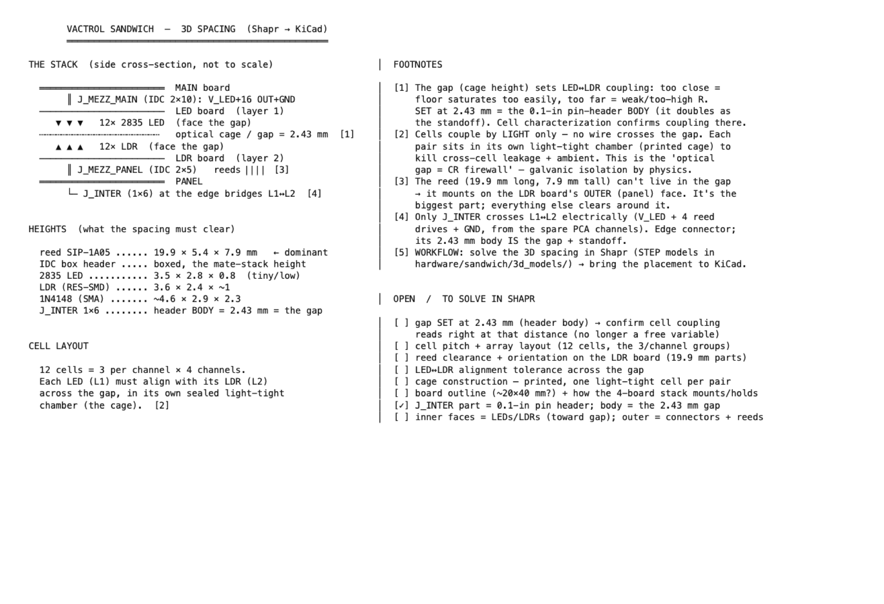 FIG. 2 — Spacing sheet for a two-board optical stack. The coupling gap is set at 2.43 mm by the body of a standard pin header, and the sheet tabulates the height of every part that has to clear it. Mechanical questions get solved at this scale, not at the soldering iron.
2. Build
Assembly is by hand, at the bench, one board at a time. The build isn’t finished when the last joint cools — it’s finished when the board is dressed: every switched position labeled with what is loaded there, so the hardware states its own configuration.
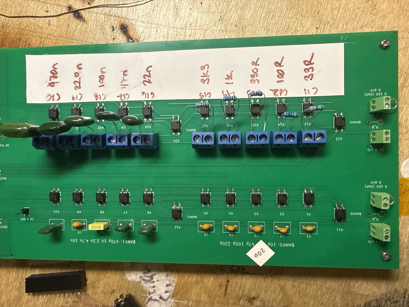 FIG. 3 — A relay-switched capacitor instrument, dressed. Twenty-four relays select values from two silkscreened banks (10 pF through 220 pF, 470 pF through 10 nF); the screw terminals hold the swappable positions, and the handwritten label strip records what each one carries right now — 470 nF down to 22 nF on one row, 3.3 kΩ down to 33 Ω on the other. When a value changes, the label changes.
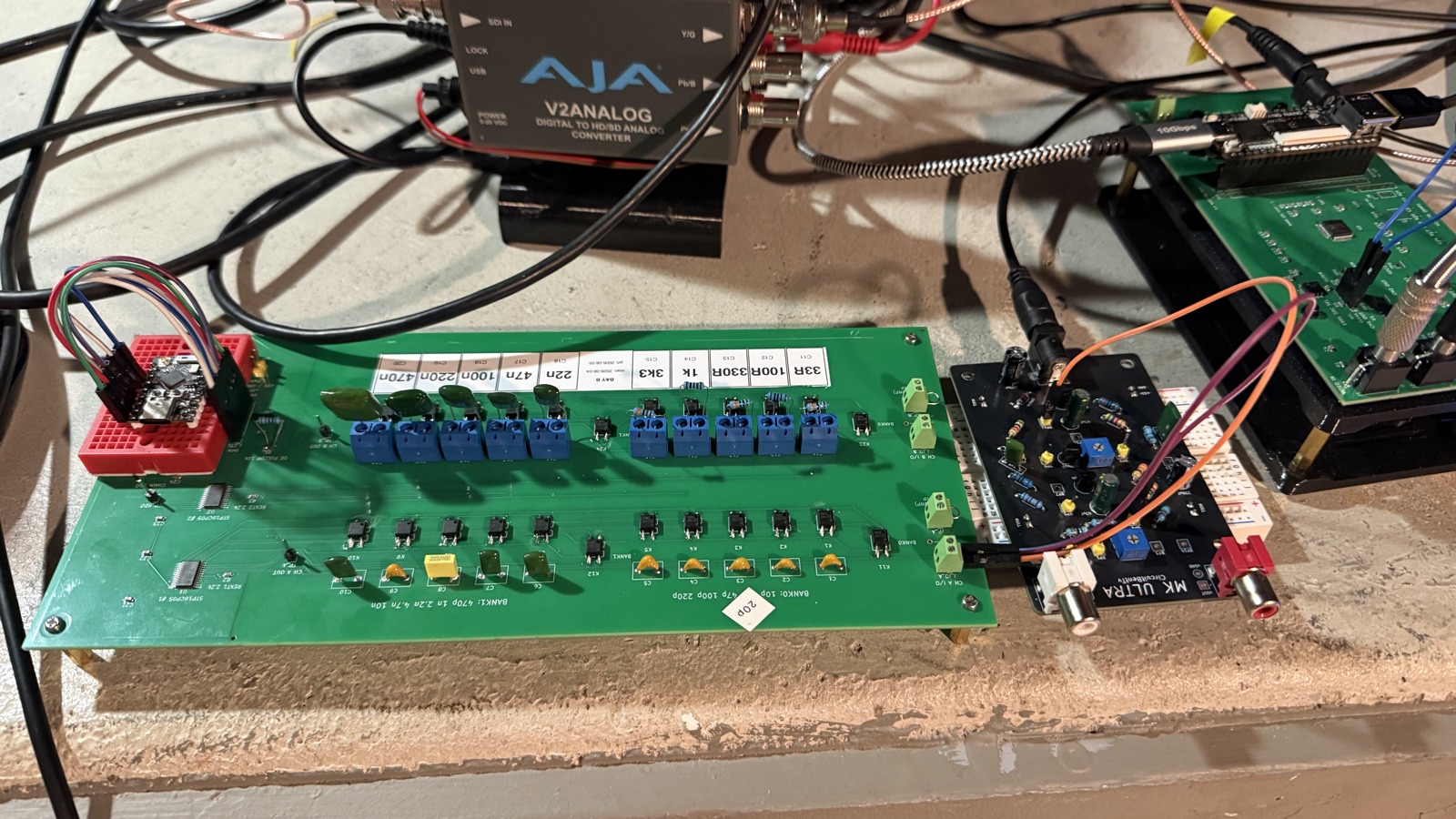 FIG. 4 — The same board in its working position: playout converter upstream, the instrument in the middle of the signal path, capture hardware downstream. Nothing here is a prop; every cable is doing something.
3. Measure
A glitch you can’t see at microsecond scale is a glitch you don’t understand. Signals through an instrument get captured raw — 13.5 megasamples per second of the composite waveform itself, not a screenshot of the picture — and decoded in software, so the same capture yields both the image and the scope trace that explains it.
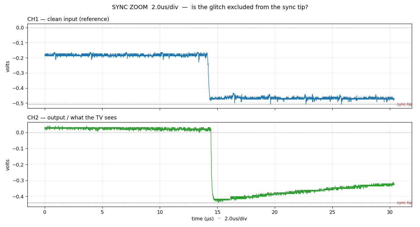 FIG. 5 — Sync zoom at 2 µs per division. Top: the clean input’s horizontal sync edge. Bottom: the instrument’s output — the edge survives, but the sync tip sags back toward blanking across the line. This is the class of defect that decides whether a display holds lock, and it is invisible until you look at this scale.
4. Catalog
Measurement feeds a catalog. Every bend an instrument can produce gets mapped: which control coordinate produces it, where its onset sits, what it looks like on the waveform, what it looks like on the screen. The catalog work is where the easy assumptions die. Onsets can be bistable — one setpoint, two different glitches, alternating. Thresholds drift with device state and history. So no setpoint gets recorded from a single visit; each one is sampled repeatedly, with settle time between reps, and the catalog records the family of states observed rather than pretending there was one.
5. Perform
Only after the map exists does the instrument get played. A mapped bend has named coordinates, a known onset, and a known recovery — which means it can be driven deliberately, held, and released, the way you’d play any instrument with a spec sheet. The performance looks like chaos. It is drawn, built, measured, and cataloged chaos, executed on demand.
That is the whole method. The drawings are engineering drawings, the measurements are measurements, the catalog is a catalog — and the output is ruin with a control law. Not broken. scientifically broken.